Everyone has their favourite data structure, and mine happens to be the trie, otherwise known as the prefix tree.
...
...
...
Hold on, before you close the tab right after reading that, I promise this blog post becomes something useful. I've never really written a blog post on a specific data structure before, so when I decided to write one it was a no brainer which one to pick.
Tries and I go way back. Once upon a time, boggle actually was a big part of my life. Every year we had this thing called inter-hall games (IHG) where people like yours truly either competed in sports or recreational games. It might seem like a waste of time, but countless friendships were forged and really I got to stay in hall for four years. (Anyone that studied at NTU can attest to how important that is!).

The Trie data structure has a special place in my little heart because it was the first time I put something theoretical to good use in my freshman year. Building a boggle solver in my first year of university helped build my confidence early on. In this blog post, I want to write about the Trie (also known as a prefix tree), and how it's implemented through various use cases. It's nothing too complex that our simple human brains can't comprehend, I promise!
Boggle's word solver
The rules of the game
In the game of boggle, players are presented with a 4x4 grid of letters. The goal of the game is to identify the most number of words given a time limit (longer words score you more points). Players can traverse vertically, horizontally or diagonally for each word without using the same letter twice. Each word must be at least 3 letters long.
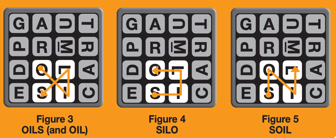
Solving the board via brute force DFS is insanity. There are 12,029,640 distinct paths to go over. A pruned solution like a trie reduces visits to a tiny fraction. Also note that the typical use case of using a hashmap does not work here because you want to know if there are words that start with a prefix, not just whether a word is in the dictionary. Even if you were to store every prefix in a hashmap, the Trie is still going to be more memory efficient because each prefix is stored only once.
Now that we understand the problem at hand, let's look at what a simplified version of the solution looks like.
Solving boggle with a Trie
A trie stores the dictionary letter by letter: each word is a path from the root, and words sharing a prefix share that path. Each node carries a flag for whether the path ending there spells a complete word.
type node struct {
children map[rune]*node
word bool
}To build a trie, we have to insert every single word in the dictionary into the trie. Insertion looks like this:
func Build(words []string) *node {
	root := &node{}
	for _, w := range words {
		root.insert(w)
	}
	return root
}
Build returns the root of the trie holding every word
func (n *node) insert(word string) {
	for _, letter := range word {
		next, ok := n.children[letter]
		if !ok {
			if n.children == nil {
				n.children = make(map[rune]*node)
			}
			next = &node{}
			n.children[letter] = next
		}
		n = next
	}
We walk the trie one letter at a time, creating the nodes as we go.
	n.word = true
}
We flag the last node as a word.
Next, let's take a look at the boggle solver's shape.
func Solve(board [][]rune, root *node) []string {
found := map[string]bool{}
We use a set to store the final set of words found on the given boggle board, because the same word can appear on different paths on the board.
	used := make([][]bool, len(board))
	for r := range used {
		used[r] = make([]bool, len(board[r]))
	}
We use a slice to store cells that have already been visited in the current explored path.
var path []rune
We also keep the path of letters so far in the spelt word. We can treat this as a shared buffer that we push and pop to.
	var dfs func(r, c int, n *node)
	dfs = func(r, c int, n *node) {
		// to be explored later
	}
DFS - this is the juicy bit, we'll come back to it later.
	for r := range board {
		for c := range board[r] {
			dfs(r, c, root)
		}
	}

	out := make([]string, 0, len(found))
	for w := range found {
		out = append(out, w)
	}
	return out // result in random order
}
Assuming we have DFS written, we solve the board by searching for words through each cell on the board. Any cell can be the start of a word.
Now to the DFS bit! The dfs function takes in the row and column values of the next cell that needs to be explored.
func Solve(board [][]rune, root *node) []string {
	// ...
	var dfs func(r, c int, n *node)
	dfs = func(r, c int, n *node) {
		if r < 0 || r >= len(board) || c < 0 || c >= len(board[r]) || used[r][c] {
			return
		}
We return early if the cell to explore has already been used or we reach the outside of the board.
		next, ok := n.children[board[r][c]]
		if !ok {
			return
		}
We return early if no word starts with the path + this letter. We essentially prune and abandon the subtree because we know no words are prefixed with the new node addition
		used[r][c] = true
		path = append(path, board[r][c])
Otherwise, we mark the cell as used, and append node to the current path.
		if next.word {
			found[string(path)] = true
		}
		for dr := -1; dr <= 1; dr++ {
			for dc := -1; dc <= 1; dc++ {
				if dr != 0 || dc != 0 {
					dfs(r+dr, c+dc, next)
				}
			}
		}
If the current node is a word, we add it to the final solution. Then we continue recursing to the 8 neighbour cells to find longer words.
		path = path[:len(path)-1]
		used[r][c] = false
	}
	// ...
}
Backtrack to release the current cell from being used, and pop the letter from the path buffer. At the end of each recursive call, we revert the board back to the state we started from.
An example usage of the code snippets so far looks something like this.
dictionary := []string{"cat", "cart", "car", "rat", "rate", "star", "arts", "tear", "seat"}
board := [][]rune{
[]rune("catd"),
[]rune("rtse"),
[]rune("aeio"),
[]rune("lnpu"),
}
fmt.Println(Solve(board, Build(dictionary)))This is how the trie actually looks like when visualised
(root)
├── a
│ └── r
│ └── t
│ └── s* arts
├── c
│ └── a
│ ├── r* car
│ │ └── t* cart
│ └── t* cat
├── r
│ └── a
│ └── t* rat
│ └── e* rate
├── s
│ ├── e
│ │ └── a
│ │ └── t* seat
│ └── t
│ └── a
│ └── r* star
└── t
└── e
└── a
└── r* tearWhen is a trie worth using?
For a dictionary averaging L letters in a word, finding out if anything is prefixed with something yields O(L). Listing all k words with a prefix yields O(L + k). Each prefix is stored in memory once only, one node per letter.
Generally, use a prefix-tree or trie if you need fast prefix-based lookups or string matching operations that are dependent on the length of the target string.
If we think about the use cases of a Trie / Prefix tree, the same problem shape shows up in a few places. What are some of these other use cases?
A quick look at HTTP routers
HTTP routers are code that live in web servers that help decide which handler function gets invoked for incoming requests. For example, in a simplistic social media backend API when a HTTP request arrives for /users/123/posts, web servers need to figure out which handler function to run.
HTTP routers must always match requests with the most specific pattern.
Before we look at a real world example, it'll be nice to understand what a Radix tree is.
Quick intro to radix trees
A radix tree is an optimized flavour of a prefix tree, where single-child nodes are merged together.
Given the same dictionary I provided in the boggle use case - a radix tree would give you the following structure.
(root) (root)
├── a-r-t-s* ├── "arts"*
├── c-a ─┬─ r* ─ t* ├── "ca" ─┬─ "r"* ─ "t"*
│ └─ t* │ └─ "t"*
├── r-a-t*-e* ├── "rat"* ─ "e"*
├── s ─┬─ e-a-t* ├── "s" ─┬─ "eat"*
│ └─ t-a-r* │ └─ "tar"*
└── t-e-a-r* └── "tear"*An example of a HTTP router that uses a radix tree is chi's HTTP router.
Real world example of a trie from go stdlib
Go 1.22 introduced enhancements to how the net/http package handles routing. This blog entry describes what was introduced. Specific code for the routing tree can be found here.
Strictly speaking, the routing tree used in go's standard library isn't a radix tree. Each symbol (or edge) in the tree represents a segment on the path. It does not follow the strict rule that radix trees have (we don't collapse/compress nodes).
You'll find routing tree's routingNode really similar to what we had for the boggle solver's prefix tree node.
type routingNode struct {
pattern *pattern // the route that ends here
handler Handler // the Handler that gets invoked
children mapping[string, *routingNode] // children nodes
multiChild *routingNode // the {rest...} catch-all
emptyChild *routingNode // a single {wildcard}
}patternis the equivalent ofwordin our prefix tree. A non-nil pattern tells us that a route ends here. AHandleralso exists on the leaf node. It's invoked when a pattern is matched.childrenmaps segments of the routes. For example for/users/bryantthere's a single child under the keyusersand one under the keybryant.emptyChildrepresents a wildcard segment. In/users/{id}, it really does not matter what the key is. Because technically/users/{userID}would also fall under the same subtree.multiChildrefers to the use case where the route is defined like this/users/{id}/posts/{path...}. It's not meant to match one segment, but matches everything that's appended at the end.
Let's say we register the following routes.
mux.HandleFunc("GET /users/bryant", ...)
mux.HandleFunc("GET /users/{id}", ...)
mux.HandleFunc("GET /users/{id}/posts/{rest...}", ...)Let's visualise the routing tree in a similar fashion, with * representing leaf nodes too. We'll get a tree like so:
(root)
└── "GET"
└── "users"
├── "bryant"* (literal, in children)
└── ""* (emptyChild: that is one segment, any value)
└── "posts"
└── "*"* (multiChild: the rest of the path)Now to the interesting bit again! Similar to what we did for the word solver, there's a recursive function that matches entire paths.
func (n *routingNode) matchPath(path string, matches []string) (*routingNode, []string) {
	if n == nil {
		return nil, nil
	}
	if path == "" {
		if n.pattern == nil {
			return nil, nil
		}
		return n, matches
	}
If there's no path left, we check if the node is a leaf node by looking
at pattern.
	seg, rest := firstSegment(path)

	if n, m := n.findChild(seg).matchPath(rest, matches); n != nil {
		return n, m
	}
Otherwise, we chop off the first segment and compare it with the literal
child first. findChild checks if the segment exists in the children
map, before invoking matchPath recursively against the rest of the
path.
	if seg != "/" {
		if n, m := n.emptyChild.matchPath(rest, append(matches, seg)); n != nil {
			return n, m
		}
	}
If no literal child matches, we then try the single wildcard child.
Whatever the segment was gets recorded as a match (with trailing slashes
skipped /).
	if c := n.multiChild; c != nil {
		matches = append(matches, pathUnescape(path[1:]))
		return c, matches
	}
Failing that, the multi-wildcard catchall gets matched to the rest of the path
	return nil, nil
}
If nothing gets matched, we return nil to the caller. The parts of the code that return nil in fact do backtracking.
How does backtracking still play its part here? Let's take an example where we registered two routes:
mux.HandleFunc("/a/b/z", handlerZ)
mux.HandleFunc("/a/{x}/c", handlerC)A request for /a/b/c will look like this:
...
segment "b" -> literal child 'b' exists, descend to the next child
segment "c" -> under 'b' there is only 'z' which is a dead end. return nil
<- unwind all the way back to 'a'
segment "b" -> no literal left, so try emptyChild. {x} = "b"
segment "c" -> match, handlerCThis is exactly what our Boggle solver was doing! Once a dead end is reached, we undo, try the next branch in the subtree. Instead of the eight neighbouring cells, this time we go for the next tier in specificity.
So far, we've looked at two flavours of Tries! One helps spell out words, one letter at a time, the other spells out URLs a segment at a time.
How small can a symbol on the Trie get? Turns out the smallest segment can be a bit.
Quick look at IP routing tables
Every device like our Macbooks for example, needs to know where to send a packet to, given an IP address. This information resides in the IP routing tables which can be found by running netstat -rn on your MacOS or ip route on Linux. Here's a trimmed version of mine:
❯ netstat -rn
Routing tables
Destination Gateway Netif
default 192.168.0.1 en0 <- anything at all
192.168.0 link#15 en0 <- my home network
192.168.0.9 aa:bb:cc:dd:11:22 en0 <- one specific machine
127 127.0.0.1 lo0 <- myself
...The Gateway field tells our device the next hop is (Another IP address if it requires forwarding, or another device on the local network). BSD uses a shorthand 192.168.0 for 192.168.0.0/24, and 127 for 127.0.0.0/8. In both cases, the first 24 and 8 bits are fixed respectively. default means 0.0.0.0/0 which matches every IP address there is.
So let's say we have a packet that needs to get to 192.168.0.9, we know from the table that 3 lines match it. The line for /32 for the exact machine, /24 for my home network, and default since it matches everything. The most specific one gets picked!
From a networking perspective, this is also known as the longest prefix match. If you haven't realised, it's the same thing we solved in the http router use case!
Using a trie to solve IP routing
The rule 192.168.0.0/24 is really just saying the first 24 bits are the prefix.
192.168.0.9 = 11000000 10101000 00000000 00001001
└─ 192 ─┘└─ 168 ─┘└─ 0 ─┘└─ 9 ─┘The problem can essentially be solved with a binary trie where there are only two symbols 0 and 1.
This works, but is makes for an odd looking tree. An IP address consists of 32 bits, so the trie becomes 32 levels deep. If we build a trie that way for the three rules from my table, we get a really long chain.
Fortunately, we've already discussed the concept of a radix tree. If we apply the same concept here where we compress edges of the tree if there's only one child we get something called a Patricia trie.
PLAIN BINARY TRIE PATH COMPRESSED
(root) default * (root) default *
│ 1 │
● bit 0 │ skip bits 0-23
│ 1 ▼
● bit 1 192.168.0.0/24 *
│ 0 │
● bit 2 │ skip bits 24-31
⋮ 21 more nodes ▼
◉ 192.168.0.0/24 * 192.168.0.9/32 *
│
⋮ 7 more nodes
◉ 192.168.0.9/32 *The command netstat -rn I mentioned earlier uses a Patricia trie in a file called radix.c that was written by Keith Sklower for BSD in 1988. This is still being shipped today! The code is old enough that it's written in a dialect of C that predates the standard that I'm more used to. Back in those days the C compiler was very different.
The core implementation idea is the same with one small caveat.
In the case of IP addresses, a more specific IP address is deeper in the tree. For example a /24 is longer than a /8. Also, if you recall, in the compressed trie, we actually deleted nodes that had nothing to decide. So if you get to the end of the tree, it's perfectly reasonable that you don't land on a matching pattern and that the solution was higher up in the tree.
This is different from how the HTTP router example worked. /users/bryant and /users/{id} are at the same tree level. It's possible for conflicts in URL routes, but this is never the case in IP addresses.
What this means is that when we reach the end of the tree, and we don't find a pattern at the end, we'll need to "climb" back up the tree for the last pattern that did match. For HTTP routes, the conditions for specificity were ordered in the go code, written by hand.
One last trie: prefix KV caches
Here's one last place where prefix trees show up. If you've used one of the managed LLM APIs recently, chances are that you've already used some form of prompt caching. OpenAI, Anthropic and Google all offer it today. The exact API and cache policy differ between providers. Some cache automatically, while others let you mark reusable prompt boundaries. However, in all cases the mental model is broadly the same.
Before an LLM generates an answer, it first has to read the prompt. This is called the prefill phase. As the model goes through the tokens, its attention layers calculate key and value vectors for them. These intermediate results are kept in a KV cache, so that the model does not have to recalculate every earlier token whenever it generates the next one.
Normally that explains how one request avoids repeating its own work. Prefix caching takes it one step further. If a new request begins with exactly the same tokens as an earlier one, the server can reuse the KV cache for the shared portion too.
Let's say we send three requests to the same coding assistant:
You are a coding assistant. Follow these rules...
├── Explain this function
├── Find the bug in this function
└── Write tests for this functionThe system prompt might be thousands of tokens long, but it is identical every time. Instead of processing all of it again, the next request can start from the cached state and continue from the point where the prompts diverge.
The cute part is that the trie is not storing words or routes this time. It is indexing work the GPU has already done.
You can probably see where this is going. We can index token sequences with a radix tree, with each cached path referring to the KV-cache blocks for that portion of the prompt:
(root)
└── "You are a coding assistant..." [cached KV]
├── "Explain" [cached KV]
├── "Find the bug" [cached KV]
└── "Write tests" [cached KV]When a new prompt arrives, the server finds the longest prefix it has already seen, reuses its cached values, then resumes computation from the first new token. Long runs of tokens with no branching can be compressed into one edge, exactly like the radix tree we saw in the HTTP router.
SGLang’s original paper called this radix-tree approach RadixAttention. It was not the first work to share KV caches across requests. What was interesting was that SGLang made finding and reusing these prefixes automatic.
The name SGLang came from Structured Generation Language. At the time, it was both a small language for writing multi-step LLM programs and a runtime for executing them efficiently. RadixAttention lived inside that runtime. It kept KV caches from previous requests in a radix tree and automatically reused the longest matching prefix.
SGLang has grown quite a bit since then. Today it is better known as an open-source serving framework for running LLMs and multimodal models. In other words, it sits on the server side and does the unglamorous work of scheduling requests, managing GPU memory and generating tokens quickly. RadixAttention is still one of the ideas at its core.
Where would this actually help? Shared system prompts are the obvious example. It also comes up with few-shot examples reused across requests, asking different questions about the same long document, and multi-turn conversations where almost the entire chat history is sent again with one new message appended.
There are two caveats. First, the tokens have to match from the beginning. Identical text buried somewhere in the middle does not count as a shared prefix. Second, this only avoids work during the prompt's prefill phase. It gets us to the first generated token sooner, but it does not make the model spit out the remaining tokens any faster.
The application may not even have to manage any of this itself. It can send the full prompt like normal, while the inference server finds the longest matching prefix and reuses whatever is still in the cache. Once again, the tricky-looking optimisation comes down to walking a tree.
The 'end' of the rabbit hole
If you reached the end of this post, I hope you gained a new found interest in the trie data structure! It's not every day I go down a rabbit hole like this one. The trie we get taught in school typically comes with 26 alphabetical symbols and a dictionary. In practice, our symbols might be letters, URL segments, bits in an IP address or tokens in an LLM prompt.
Turns out that quite a few problems become a tree once you ask: "How much of this beginning have I seen before?"